Be sure to check out the previous two posts:

1. Hemispherical Light Estimates

2. Hardware for Hemispherical Photos

Once the theory and equipment are taken care of, you are ready to go out into the field and collect data. This post will cover the when, where, and how of shooting hemispherical photos. The next and final post deals with analyzing the photos you’ve captured.

When:

Hemispherical photos are very sensitive to lighting conditions. Because you are measuring an entire half hemisphere of the sky at once with each photo, it is important that the background (i.e. the sky) is as standardized as possible so that the canopy can be accurately distinguished without bias.

To imagine the wildly different exposures gradient across a hemispherical lens, wait until a clear sunset and walk out into an open field. Stare directly at the setting sun for a few seconds, then turn 180 degrees and try to make out the horizon. Even though our eyes are extremely well-equipped to quickly adjust for different lighting, you’ll probably have a hard time making out the dark horizon after looking at the bright sunset. Unlike your eye, which continuously adjusts to light conditions even at these extremes, cameras are stuck in one setting. Even the best camera sensors are limited in their tolerances, so we need to take photos at times when lighting in the entire hemisphere fits within a narrow range.

The best time to shoot is on uniformly overcast days. Overcast cloud cover yields a nice homogeneous white background that makes strong contrast to the edges of leaves and branches.

If cloudy days are not in the forecast, another option is to wait until dawn or dusk, before or after the sun is below the horizon and the sky is evenly lit. The problem is that this only allows a very short window for shooting.

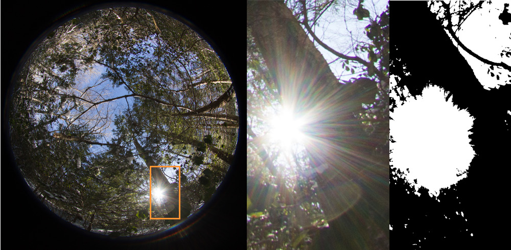
Sometimes, we can’t help but take photos on sunny days. Before I talk about strategies for dealing with difficult exposures, I want to explain some of the problems direct sunlight can precipitate in light estimation methods: blown-out highlights, flare, and reflection.

Overexposed highlights

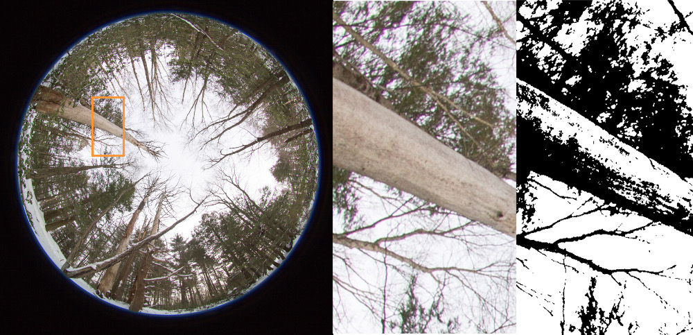
Overexposed or “blown-out” highlights is an issue of exposure settings and sensor limitations. When shooting into light, individual sensor cells can only record light up to a threshold. In my last post, I compared light collecting on camera sensor cells to an array of buckets in a field collecting raindrops. Using that analogy, think about sensor thresholds as the rim of the bucket. At some point, enough rain collects in the buckets that it overfills. After that point, you can record no more information about relative rainfall between buckets. In the camera, eventually too much light falls incident on a portion of the sensor and those pixels are maxed out and recorded as fully white (i.e. no information is coded in those cells). This leads to an underestimate of canopy closure because some pixels occupied by canopy will look like white sky after binarization. We can try correct our exposure to ensure we do not truncate those bright pixels, but compared to direct sun, blue sky directly overhead is relatively dark on sunny days, so this will almost certainly lead to a loss of information on the dark end of the spectrum, and we will then be overestimating canopy closure.

Unfortunately, there are no easy ways to deal with wide exposure ranges (other than avoiding sunny days). One solution is to shoot in RAW format which retains more information per pixel. With RAW photos one can attempt to recover highlights and boost shadows to some extent, but because the next processing step is binarization, this will only be effective if you can sufficiently expand the pixel value range at the binarization threshold. This also entails hand-calibrating each image, which reduces standardization and replicability, and may take a lot of time if you need to process many photos.

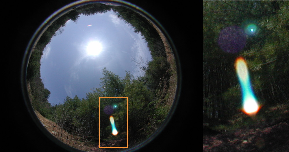
Flare

Flare is another problem and it emerges for a couple of reasons.

Hazy-looking “veiling flare” occurs when light scatters inside the glass optics of your lens. In normal photography, it is most prevalent when the sun is oblique to the front lens surface and light gets “trapped” bouncing around inside of the glass. It can also look like a halo of light bleeding into a solid object or streaks of light radiating from a point of light depending on your aperture settings (this is called Fraunhofer diffraction and can make for very cool effects…just not in hemispherical photos!). When these streaks appear to overlay solid canopy objects in our photos it will lead to underestimation of closure.

Ghosting flare looks like random orbs of light in photos and it occurs when light entering the lens highlights the inside of the optics close enough to focus on the sensor. Hemispherical lenses are incredibly prone to this type of flare because of the short focal distance of wide angle lenses.

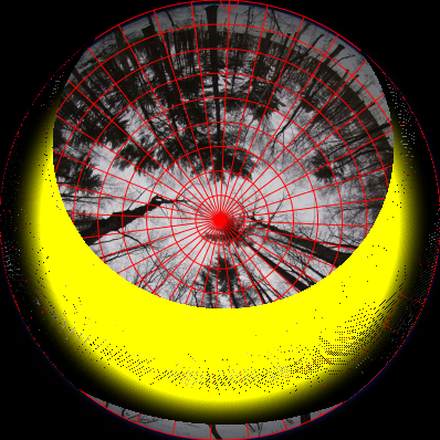
If photos must be taken in sunlight, one alternative is to at least block the direct beams of sunlight by positioning the sun behind a natural sunblock or fashioning a shield. I’ve never tried the shield option myself, but I’ve seen photos of folks who have affixed a small disk on a semi-ridge wire on their tripod. The disk can be positioned such that it only blocks the sun. There are many problems with this option. First, the sunshield will be counted as canopy in the light calculations which will bias the estimates. One could exclude the blocked area from analysis by masking out the area of interest, but then that area will be excluded from the analysis. Another option is to spot-correct flare in each photo. This is most effective with RAW photos and can be accomplished in photo-editing applications by using a weak adjustment brush to reduce highlights, boost shadows, and increase contrast directly over the flare. Again, I don’t recommend editing individual photos, but sometimes this is the only option.

Reflection

Finally, direct sun reflecting on solid surfaces can lead to mischaracterization of pixels and overestimate openness. In this case, objects opposite the sun can be lit so well that they are brighter than the background. This is very common in forests dominated by light bark trees like aspen and birch. This also occurs just about any time there is snow in the frame, regardless of the lighting conditions. The only solution for this problem is darkening the solid objects in a photo-editing program. It is a painstaking task and increases the error in the final estimation, but sometimes is necessary.

Where.

Next you must decide where you want to take photos. The answer to this will depend on your research question. We can break it down into spatial/temporal sampling scale and relative position.

Hemispherical photos can fit into any standard spatial sampling scheme (e.g. transects, grid, opportunistic, clustered, etc.) depending on your downstream statistical analysis. However, because hemispherical photos capture such a wide angle of view, you must be careful of any analysis that assumes independence of observations if the viewshed overlaps between photos.

Generally, when we think about spatial sampling, we think in two dimensions (like in the figure below). However, it is also important to consider that canopy closure estimates integrate sun angle, and so it is critical that an even sampling scheme considers the third spatial dimension and include a representative sample of topographical aspect.

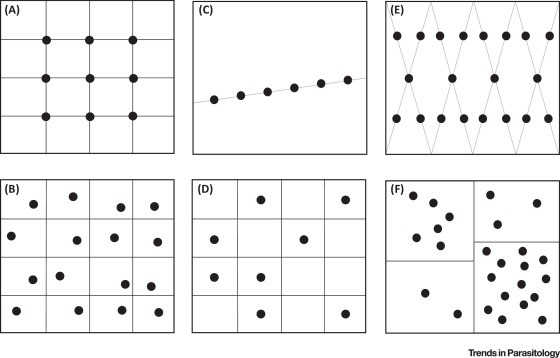
There is no perfect sampling strategy for any given project. To illustrate some considerations, I will outline the sampling for my work. For my project, I need to characterize the canopy closure above forested pond that range in size from a few meters to a hundred meters across. The most obvious strategy was to sample the intersections of a tightly spaced Cartesian grid over the entire surface of the pond. A previous research student tried this method on a handful of ponds. Using that information, we were then able to subsample those data to determine the spacing of the grid that would yield the most accurate estimates with the fewest photos. In this case, it turned out that every pond, regardless of size, could be characterized with 5 photos: 4 photos along the most distal shoreline in each cardinal direction and one photo in the center of the pond where the east-west and north-south lines intersect. An ancillary benefit of taking the same number of photos at each pond is that I can also calculate the variance within each pond, which gives me a sense of the homogeneity of the habitat. Keep in mind that measures of higher moments of the distribution of light values across habitats (like variance or kurtosis) may be extremely ecologically relevant and can be incorporated for more meaningful statistical analysis.

One final consideration in spatial sampling is the height at which photos are captured. By virtue of practicality, the most common capture height is about 1m from the ground since this is the height of most tripods. However, the study question might dictate taking photos above understory plants or at ground level. Regardless, the height of photos should be consistent, or recorded for each photo, and explicitly stated in published methods.

You will also need to consider the frequency of your sampling to ensure that you capture any relevant variation in the study system over time. In temperate forests, this usually means, at the very least, taking the same photos with deciduous leaves on and again after the leaves have fallen. On the other hand, phenological studies might need photos from many timepoints over shorter durations.

It is important to remember that canopy closure estimation integrates the sun’s path over a specific yearly window. We will define that window explicitly in the model, so it is important to ensure that the canopy structure in the photos accurately represents the sunpath window you define.

How.

In this section I will get into the nuts and bolts of taking photos in the field. I’ll cover camera settings and then camera operation.

Camera settings.

Most modern cameras are designed for ease of use and offer a variant of “automatic” settings. Automatic settings are great for snapping selfies and family photos, but awful for data collection. Manually adjusting the camera increases replicability and increases the accuracy of light estimates. Fortunately, there are only 4 parameters that we need to adjust for hemispherical photography: ISO, aperture, shutter speed, and focal distance.

ISO measures the sensitivity of a camera’s sensor to light. Higher ISO settings ( = greater sensitivity) allow for faster capture in lower light. However, high ISO leads to lots of noise and mischaracterization of pixels. In general, you should aim for the lowest ISO setting possible to produce better quality photos. More expensive cameras have better sensors and interpolation algorithms, so you can get away with higher ISO settings.

The aperture is the iris of a lens and controls the amount of light entering the camera. Aperture settings are given in f-numbers (which is the ratio of the lens focal length to the physical aperture width). Counterintuitively, a larger f-value (i.e. f22) is a smaller physical pupil, and therefore, less light than a smaller f-value (i.e. f2.8). Your aperture settings will be a balance between letting in enough light and getting crisp focus across the focal range (see focal distance below).

The shutter speed determines the duration of time that the sensor is exposed to light. Longer shutter speeds means more light resulting in brighter photos. However, the longer the shutter speed, the more any movement of the camera or the canopy will blur the image. If you are using a handheld system, I suggest at least 1/60sec shutter. With a tripod, shutter speeds can be longer, but only if the canopy is completely still. If there is ANY wind, I suggest at least 1/500sec shutter.

Focal distance is the simplest—just adjust the lens focus so that canopy edges are in sharp focus. This is easy when the canopy is a consistent distance from the lens, but can be difficult when capturing multi-layer structure. Lenses resolve greater depth of field (range of focal distances simultaneously in focus) when the aperture is smallest.

Since all four settings rely on all of the others, camera settings will be a balancing act. The end goal is to ensure that you have the best balance between overly white and overly black pixels and you can check this with your camera’s internal light meter. The big catch here is that we are actually not that interested in the exposure of the sky; in fact, we would like for the sky to be entirely white.

The most common exposure standardization technique is to first determine the exposure settings for open sky, then overexpose the image by 2-3 exposure values (EV) (Beckshäfer et al. 2013, Brown et al. 2000, Chianucci and Cutini 2012). In theory, this will ensure that a uniformly overcast sky is entirely white without blowing-out the canopy. The primary benefit is that this method uses the sky as a relative reference standard which is replicable.

It is easy to employ this method using your camera’s internal light meter. First, set your camera to meter from a single central point (you will probably need to look in your manual to figure out how to do this). If there is a large enough gap in the canopy overhead, you can point the meter spot there and take a reading then adjust your settings to get a 0 EV. (If the canopy has no gaps, you can set this in the open before going into the forest–just remember to take another reading if the conditions change). Now, reduce the shutter speed by 2 full stops (i.e. if 1/500 is 0 EV for the sky, set your shutter speed to 1/125; if 0 EV is 1/1600, set you speed to 1/400).

[Note, other authors (e.g. Beckshäfer et al. 2013) suggest adjusting for 2 EV overexposure. I don’t like using EV for anything other than the spot reference because all cameras use different methods of evaluating exposure. In contrast, shutter speed is invariant across all camera platforms.]

This may all seem like a confusing juggling act, but it is not that difficult in practice. Here is my general strategy:

• I set my ISO at 200 and my aperture at around f11.
• With the camera set to evaluate the central point of the image, I take a light meter reading of open sky.
• I adjust my shutter speed to an exposure value of 0 for open sky.
• Now, I re-adjust my shutter speed slower by 2 full stops.
• If my shutter speed is now too slow, I will increase my ISO one level or decrease my f-stop (aperture) by one stop and go back to step #2. I repeat until I find the balance.
• With the camera set, I can set up my camera and take images using these same settings; however, I must re-calibrate if the sky conditions change.

Taking photos.

At this point, shooting the photos is the easy part! A couple of helpful tips will make life easier.

Before shooting, you will need to orient the camera so that the sensor is perpendicular to the zenith angle (i.e. the camera lens is pointing directly up, opposite gravity). In my previous post covering hardware I mentioned that there are pre-fabricated leveling systems available or you can make a DIY version. With a tripod, you can manually level the camera.

For later analysis, you will need to know the compass orientation of the photos. Some pre-fab systems have light-up LEDs around the perimeter that are controlled by an internal compass and always light north. Otherwise, you can place a compass on your stabilizer or tripod and point the top of the image frame in a consistent direction (magnetic or true north is fine, just make sure you are consistent and write down which one you use).

It can be hard to take a hemispherical photo without unintentionally making self-portraits. With a tripod, you can use a remote to release the shutter from a distance or from behind a tree. Camera manufacturers make dedicated remotes, or if your camera has wifi capabilities, you can use an app from your phone. Most cameras also have a timer setting which can give you enough time to duck for cover.

 

Be sure to check out my other posts about canopy research that cover the theory, hardware, field sampling, and analysis pipelines for hemispherical photos.

Also, check out my new method of canopy photography with smartphones and my tips for taking spherical panoramas.

 

References

Beckschäfer, P., Seidel, D., Kleinn, C., and Xu, J. (2013). On the exposure of hemispherical photographs in forests. iForest 6, 228–237.

Brown, P. L., Doley, D., and Keenan, R. J. (2000). Estimating tree crown dimensions using digital analysis of vertical photographs. Agric. For. Meteorol. 100, 199–212.

Chianucci, F., and Cutini, A. (2012). Digital hemispherical photography for estimating forest canopy properties: Current controversies and opportunities. iForest – Biogeosciences and Forestry 5.

Collender, P. A., Kirby, A. E., Addiss, D. G., Freeman, M. C., and Remais, J. V. (2015). Methods for Quantification of Soil-Transmitted Helminths in Environmental Media: Current Techniques and Recent Advances. Trends Parasitol. 31, 625–639.