When I first developed the method to estimate canopy metrics from smartphone spherical panoramas, I used a somewhat convoluted workflow involving command line image manipulation, a plugin for ImageJ to do binarization, and a script I wrote in AutoHotKey language to automate mouse clicks on a GUI for canopy measures. Admittedly, it is a difficult pipeline for others to easily replicate.

In an effort to make life easiest, I spent some time building out the pipeline entirely in R, including a sourceable function for converting spherical panos to hemispherical images (all available on this repo).

The easiest way to convert all of your spherical panos to hemispherical projections is to source the function from my github:

source("https://raw.githubusercontent.com/andisa01/Spherical-Pano-UPDATE/main/Spheres_to_Hemis.R")

When you source the script, it will install and load all necessary packages. It also downloads the masking file that we will use to black out the periphery of the images.

The script contains the function convert_spheres_to_hemis, which does exactly what is says. You’ll need to put all of your raw spherical panos into a subdirectory within your working directory. We can then pass the path to the directory as an argument to the function.

convert_spheres_to_hemis(focal_path = "./raw_panos/")

This function will loop through all of your raw panos, convert them to masked, north-oriented upward-facing hemispherical images and put them all in a folder called “masked_hemispheres” in your working directory. It will also output a csv file called “canopy_output.csv” that contains information about the image.

Below, I will walk through the steps of the workflow that happened in the convert_spheres_to_hemis function. If you just want to use the function, you can skip to the analysis. I’ve also written a script to do all of the conversion AND analysis in batch in the repo titled “SphericalCanopyPanoProcessing.R”.

library(tidyverse) # For data manipulation
library(exifr) # For extracting metadata

R is not really the best tool for working with image data. So, we’ll use the magick package to call the ImageMagick program from within R.

library(magick) # For image manipulation
# Check to ensure that ImageMagick was installed.
magick_config()$version

You should see a numeric version code like ‘6.9.12.3’ if ImageMagick was properly installed.

# ImageR also requires ImageMagick
library(imager) # For image display

For binarizing and calculating some canopy metrics, we will use Chiannuci’s hemispheR package, which we need to install from the development version.

library(devtools)
devtools::install_git("https://gitlab.com/fchianucci/hemispheR")
library(hemispheR) # For binarization and estimating canopy measures

To get started, you’ll need to have all of your raw equirectangular panoramas in a folder. I like to keep my raw images in a subdirectory called ‘raw_panos’ within my working directory. Regardless of where you store your files, set the directory path as the focal_path variable. For this tutorial we’ll process a single image, but I’ve included scripts for batch processing in the repo. Set the name of the image to process as the focal_image variable.

focal_path <- "./raw_panos/"
focal_image <- "PXL_20230519_164804198.PHOTOSPHERE_small.jpg"

focal_image_path <- paste0(focal_path, focal_image)
focal_image_name <- sub("\\.[^.]+$", "", basename(focal_image_path))

Let’s take a look at the equirectangular image.

pano <- image_read(focal_image_path)
pano # Visualize the pano

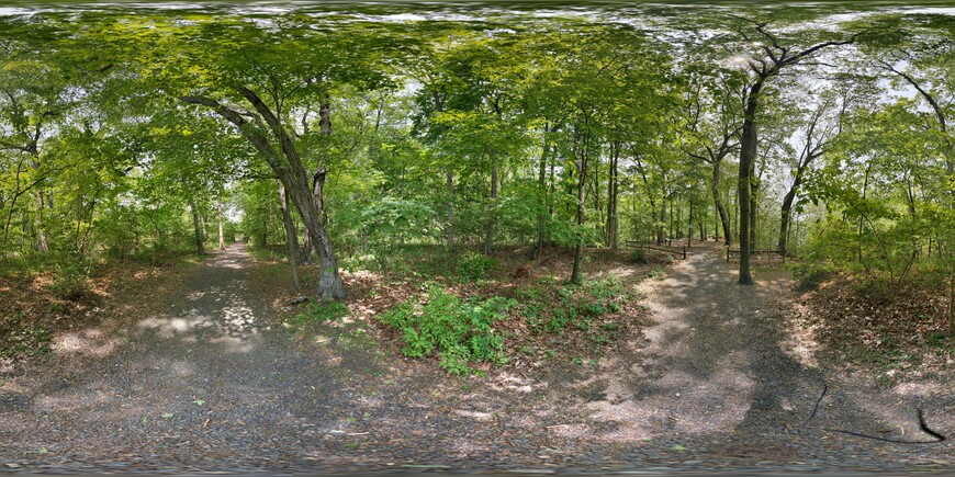
Note: One advantage of spherical panos is that they are large, and therefore, high resolution. The images from my Google Pixel 4a are 38 mega pixels. For this tutorial, I downsized the example pano to 10% resolution to make processing and visualizing easier. For your analysis, I’d recommend using full resolution images.

Spherical panoramas contain far more metadata than an average image. We can take a look at all of this additional information with the read_exif function.

read_exif(focal_image_path) %>%
  glimpse()

We’ll extract some of this information about the image, the date it was created, the georeference, and altitude, etc. to output alongside our canopy metrics. You can decide which elements are most important or useful for you.

xmp_data <- read_exif(focal_image_path) %>%
  select(
    SourceFile,
    Make,
    Model,
    FullPanoWidthPixels,
    FullPanoHeightPixels,
    SourcePhotosCount,
    Megapixels,
    LastPhotoDate,
    GPSLatitude,
    GPSLongitude,
    GPSAltitude,
    PoseHeadingDegrees
  )

The first image processing step is to convert the equirectangular panorama into a hemispherical image. We’ll need to store the image width dimension and the heading for processing. The pose heading is a particularly important feature that is a unique advantage of spherical panoramas. Since the camera automatically stores the compass heading of the first image of the panorama, we can use that information to automatically orient all of our hemispherical images such that true north is the top of the image. This is critical for analyses of understory light which requires plotting the sunpath onto the hemisphere.

# Store the pano width to use in scaling and cropping the image
pano_width <- image_info(pano)$width
image_heading <- read_exif(focal_image_path)$PoseHeadingDegrees

The steps to reproject the spherical panorama into an upward-looking hemispherical image go like this:

Crop the upper hemisphere (this is easy with smartphone spheres because the phone’s gyro ensures that the horizon line is always the midpoint of the y-axis).

Rescale the cropped image into a square to retain the correct scaling when reprojected into polar coordinate space.

Project into polar coordinate space and flip the perspective so that it is upward-looking.

Rotate the image so that the top of the image points true north and crop the image so that the diameter of the circle fills the frame.

We can accomplish all of those steps with the code below.

pano_hemisphere <- pano %>%
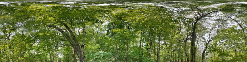
  # Crop to retain the upper hemisphere
  image_crop(geometry_size_percent(100, 50)) %>%
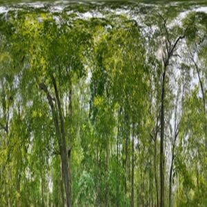
  # Rescale into a square to keep correct scale when projecting in to polar coordinate space
  image_resize(geometry_size_percent(100, 400)) %>%
  # Remap the pixels into polar projection
  image_distort("Polar",
                c(0),
                bestfit = TRUE) %>%
  image_flip() %>%
  # Rotate the image to orient true north to the top of the image
  image_rotate(image_heading) %>%
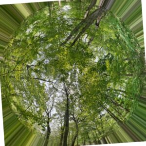
  # Rotating expands the canvas, so we crop back to the dimensions of the hemisphere's diameter
  image_crop(paste0(pano_width, "x", pano_width, "-", pano_width/2, "-", pano_width/2))

The resulting image looks funny because the outer pixels are extended by interpolation and we’ve rotated the image which leaves white space at the corners. Most analyses define a bounding perimeter to exclude any pixels outside of the circular hemisphere; so, the weird border shouldn’t matter. But, we can add a black mask to make the images look better.

I’ve included a vector file for a black mask to lay over the image in the repo.

# Get the image mask vector file
image_mask <- image_read("./HemiPhotoMask.svg") %>%
  image_transparent("white") %>%
  image_resize(geometry_size_pixels(width = pano_width, height = pano_width)) %>%
  image_convert("png")

masked_hemisphere <- image_mosaic(c(pano_hemisphere, image_mask))

masked_hemisphere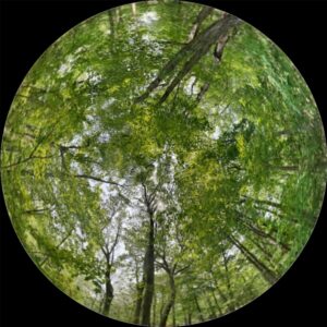

We’ll store the masked hemispheres in their own subdirectory. This script makes that directory, if it doesn’t already exists and writes our file into it.

if(dir.exists("./masked_hemispheres/") == FALSE){
  dir.create("./masked_hemispheres/")
} # If the subdirectory doesn't exist, we create it.

masked_hemisphere_path <- paste0("./masked_hemispheres/", focal_image_name, "hemi_masked.jpg") # Set the filepath for the new image

image_write(masked_hemisphere, masked_hemisphere_path) # Save the masked hemispherical image

At this point, you can use the hemispherical image in any program you’d like either in R or other software. For this example, I’m going to use Chiannuci’s hemispheR package in order to keep this entire pipeline in R.

The next step is to import the image. hemispheR allows for lots of fine-tuning. Check out the docs to learn what all of the options are. These settings most closely replicate the processing I used in my 2021 paper.

fisheye <- import_fisheye(masked_hemisphere_path,
                          channel = '2BG',
                          circ.mask = list(xc = pano_width/2, yc = pano_width/2, rc = pano_width/2),
                          gamma = 2.2,
                          stretch = FALSE,
                          display = TRUE,
                          message = TRUE)

Now, we need to binarize the images, converting all sky pixels to white and everything else to black (at least as close as possible). Again, there are lots of options available in hemispheR. You can decides which settings are right for you. However, I would suggest keeping the zonal argument set to FALSE. The documentation describes this argument as:

zonal: if set to TRUE, it divides the image in four sectors
(NE,SE,SW,NW directions) and applies an automated classification
separatedly to each region; useful in case of uneven light conditions in
the image

Because spherical panoramas are exposing each of the 36 images separately, there is no need to use this correction.

I also suggest keeping the export argument set to TRUE so that the binarized images will be automatically saved into a subdirectory named ‘results’.

binimage <- binarize_fisheye(fisheye,
                 method = 'Otsu',
                 # We do NOT want to use zonal threshold estimation since this is done by the camera
                 zonal = FALSE,
                 manual = NULL,
                 display = TRUE,
                 export = TRUE)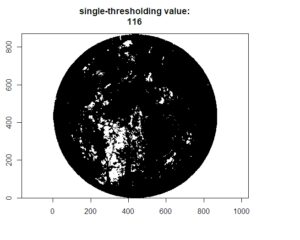

Unfortunately, hemispheR does not allow for estimation of understory light metrics like through-canopy radiation or Global Site Factors. If you need light estimates, you’ll have to take the binarized images and follow my instructions and code for implementing Gap Light Analyzer.

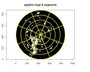
Assuming all you need is canopy metrics, we can continue with hemispheR and finalize the whole pipeline in R. We estimate canopy metrics with the gapfrac_fisheye() function.

gapfrac <- gapfrac_fisheye(
  binimage,
  maxVZA = 90,
  # Spherical panoramas are equidistant perforce
  lens = "equidistant",
  startVZA = 0,
  endVZA = 90,
  nrings = 5,
  nseg = 8,
  display = TRUE,
  message = TRUE
)

Finally, we can estimate the canopy metrics with the canopy_fisheye() function, join those to the metadata from our image, and output our report.

canopy_report <- canopy_fisheye(
  gapfrac
)

output_report <- xmp_data %>%
  bind_cols(
    canopy_report
  ) %>%
  rename(
    GF = x,
    HemiFile = id
  )

glimpse(output_report)

Rows: 1
Columns: 32
$ SourceFile            "./raw_panos/PXL_20230519_164804198.PHOTOSPHERE_small.jpg"
$ Make                  "Google"
$ Model                 "Pixel 4a"
$ FullPanoWidthPixels   8704
$ FullPanoHeightPixels  4352
$ SourcePhotosCount     36
$ Megapixels            0.37845
$ LastPhotoDate         "2023:05:19 16:49:57.671Z"
$ GPSLatitude           41.33512
$ GPSLongitude          -72.91103
$ GPSAltitude           -23.1
$ PoseHeadingDegrees    86
$ HemiFile              "PXL_20230519_164804198.PHOTOSPHERE_smallhemi_masked.jpg"
$ Le                    2.44
$ L                     3.37
$ LX                    0.72
$ LXG1                  0.67
$ LXG2                  0.55
$ DIFN                  9.981
$ MTA.ell               19
$ GF                    4.15
$ VZA                   "9_27_45_63_81"
$ rings                 5
$ azimuths              8
$ mask                  "435_435_434"
$ lens                  "equidistant"
$ channel               "2BG"
$ stretch               FALSE
$ gamma                 2.2
$ zonal                 FALSE
$ method                "Otsu"
$ thd                   116

Be sure to check out my prior posts on working with hemispherical images.