Now that you’ve got the theory, equipment, and your own hemispherical photos, the final steps are processing the photos and generating estimates of canopy and light values.

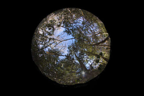
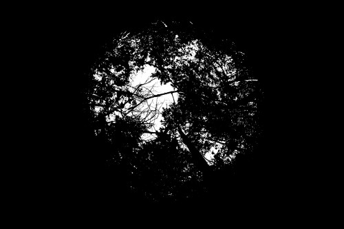
We’ll be correcting photos and then converting to a binary image for analysis just like those in the slider above.

There are many paths to get light estimates from photos. Below, I’ve detailed my own pipeline which consists of these main steps:

• Standardizing exposure and correcting photos
• Binarization
• File conversion
• Model configuration
• Analyzing images

For this pipeline, I use Adobe Lightroom 5 for standardizing the photos and masking, ImageJ with Hemispherical 2.0 plugin for binarization and image conversion, Gap Light Analyzer (GLA) for estimating light values, and AutoHotKey for automating the GLA GUI. All of these programs, with the exception of Lightroom, are freely available. You could easily replicate all of the steps I show for Lightroom in GIMP, an open-source graphics program.

There are probably stand-alone proprietary programs out there that can analyze hemispherical photos in a more streamlined manner within a single program, but personally, I’m willing to sacrifice some efficiency for free and open-source methods.

1. Standardizing photos:

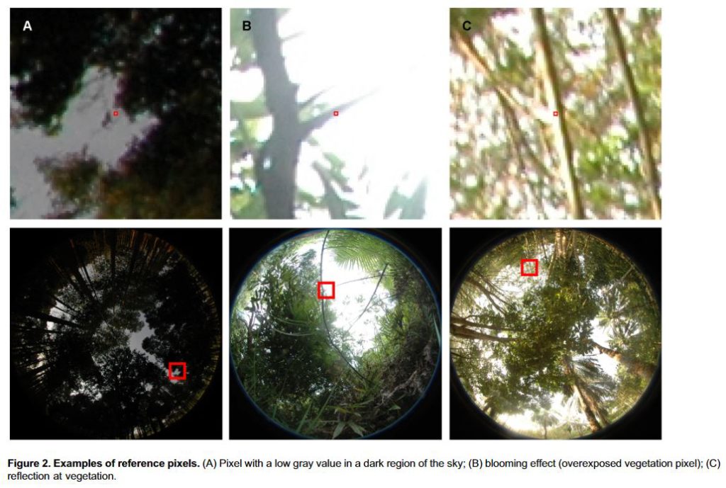
With the photos on your computer, the first step is to standardize the exposure. In theory, exposure should be standardized in the field by calibrating reference exposure to the open sky (as outlined in my previous post). However, when taking many photos throughout the day, or on days with variable cloud cover, there will be variation in the photos. Similarly, snowy days or highly reflective vegetation can contribute anomalies in the photos. Fortunately, you can reduce much of this variability in post-processing adjustments. We will apply some of these adjustments across the entire image and others we will need to correct targeted elements within the image.

Across the entire image, we can right-shift the exposure histogram so that the brightest pixels in the sky are always fully white. This standardizes the sky to the upper end of the brightness distribution across the image. So, even if we capture one photo with relatively dark clouds and another with relatively bright clouds over the course of a day, after standardizing, the difference between the white sky and dark canopy will be consistent.

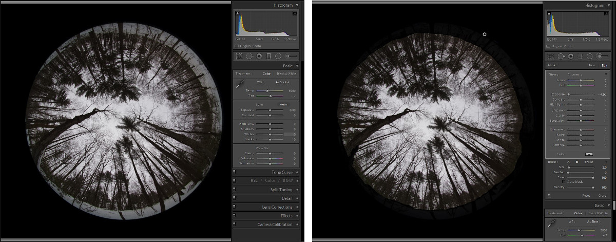
If elements of the image are highly reflective, an additional step to mask these areas is required to avoid underestimating canopy closure. For instance, extremely bright tree bark or snow on the ground should be masked. I do this by painting a -2EV exposure brush over the area to ensure it will be converted to black pixels in the binarization step. Unfortunately, this must be done by hand on each photo.

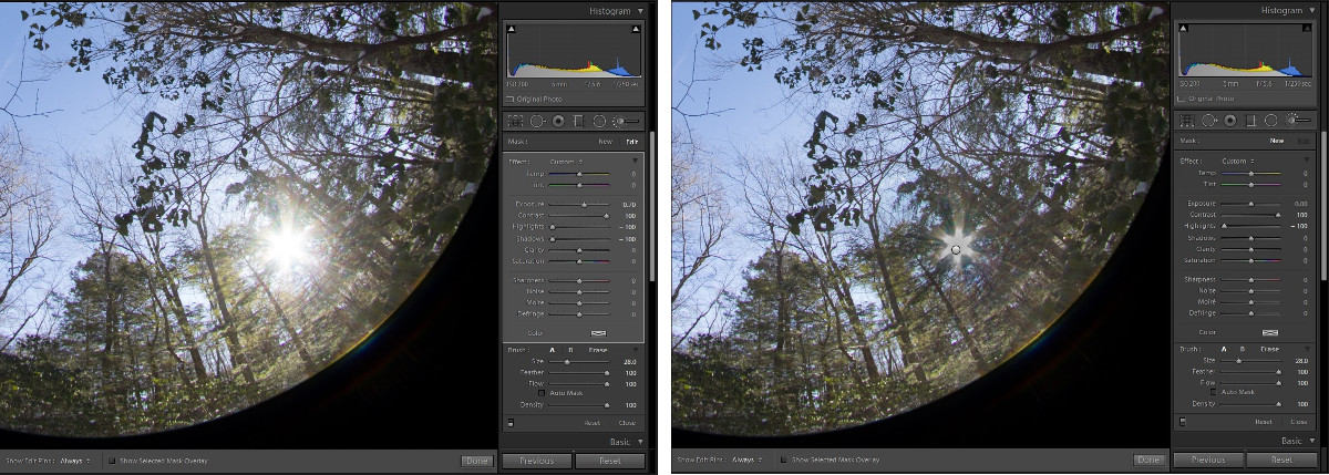
Sunspots can also be partially corrected, but again, it requires manipulation by hand on each photo. I find that a local exposure brush that depresses the highlights and increases the contrast will recover pixel that have been overexposed due to sun flare, but only to an extent. It is best to avoid flare in the first place (see my last post for tips for avoiding flare).

2. Binarization

Binarization is the process of converting all color pixels in an image to black (canopy) and white (sky). The most basic method of conversion is to set a defined threshold for the tone of each pixel above which a pixel is converted to white and below which it is converted to black. This type of simple thresholding suffers from problems in cases when pixels are ambiguous, especially at the edges of solid canopy objects. To avoid these problem, a number of algorithms have been developed that take a more complex approach. I won’t go into details here, but I suggest reading Glatthorn and Beckshafer’s (2014).

I explored a number of binarization programs while developing my project, including SideLook 1.1  (Nobis, 2005) and the in-program thresholding capability in Gap Light Analyzer (Frazer et al. 2000). However, both of these programs fell short of my needs. In the end, I found the Hemispherical 2.0 plugin (Beckshafer 2015) for ImageJ to be most useful because it is easily able to handle batch processing.

You can download the Hemispherical 2.0 plugin and manual here (scroll to the bottom of the page under “Forest Software”). This plugin uses a “Minimum” thresholding algorithm on the blue color plane of the image (skies are blue, so the blue plane yields the highest contrast). The threshold is based on a histogram populated from a moving window of neighboring pixel values to ensure continuity of canopy edges (see Glatthorn & Beckshafer 2014 for details).

Once the plugin is installed, you can run the binarization process in batch on a folder containing all of your adjusted hemispherical photo files. I’ve found the program lags if I try to batch process more than 100 photos at a time; so, I suggest splitting datasets into multiple folders with fewer than 100 files if you are processing lots of photos.

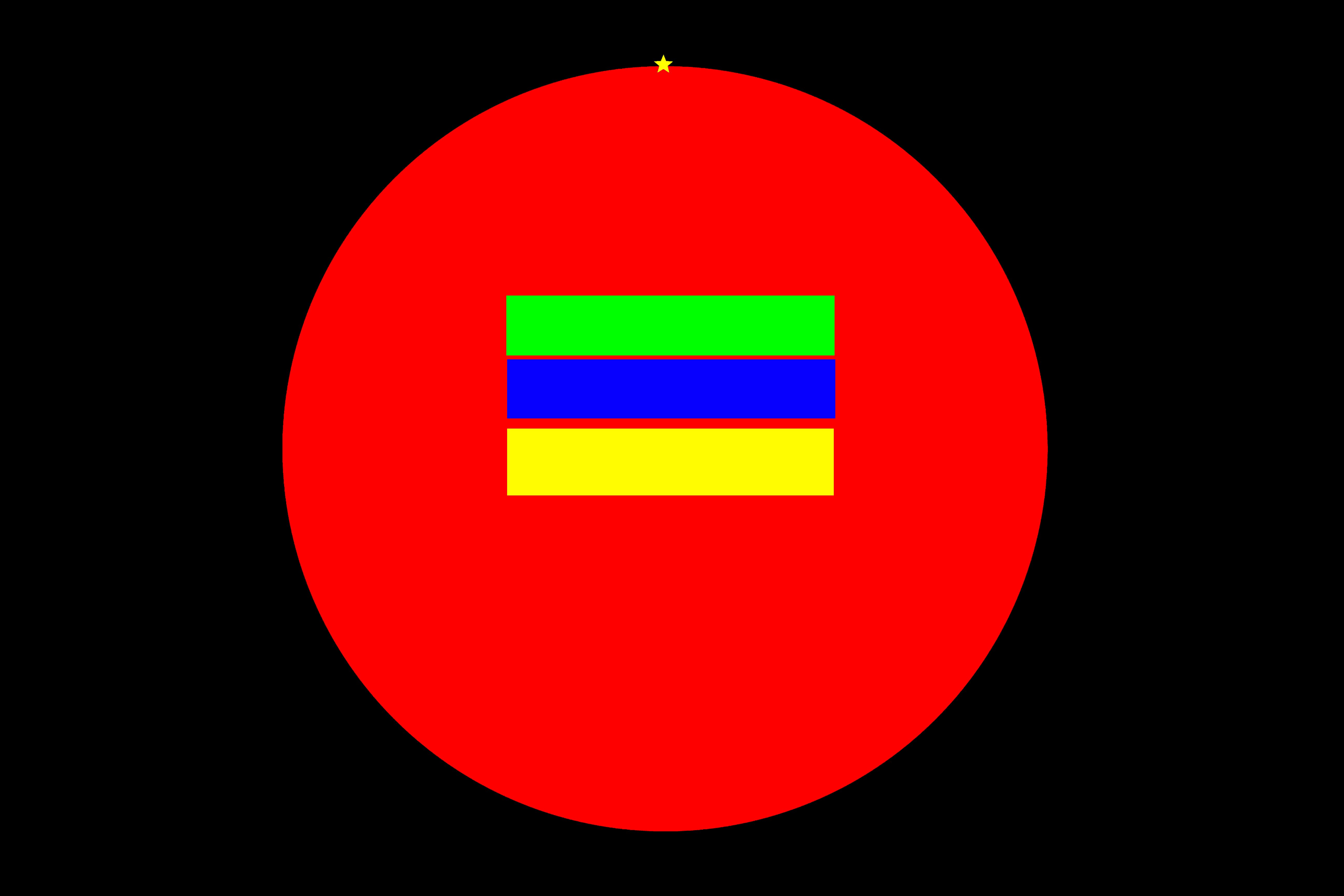
Before you begin the binarization and analysis process, I suggest that you make a registration image. The first step in both of the binarization and analysis programs is defining the area of interest in the image that excludes the black perimeter. This can be hard to do depending on which photo is first in the stack (for instance, if the ground is very dark and blends into the black perimeter). A registration image allows you to easily and consistently define your area of interest. I like to make a standardized registration image for all of my camera/lens combinations.

The easiest way to make a registration image is to simply take a photo of a white wall and increase the contrast in an editing program until you have hard edges. Or, you can overlay a solid color circle that perfectly matches the bounds of the hemisphere (as I’ve done in the photo above). I also like to include a demarcated point that indicates a Northward orientation (this is at the top of the circle, in my case). I use this mark as a starting point for manually dragging the area-of-interest selection tool in both GLA and Hemispherical 2.0.

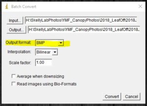
3. File Conversion

Hemispherical 2.0 outputs binarized images as TIFF files, but GLA can only accept bitmap images. So, we need to convert the binary images to bitmap files. This can easily be accomplished in ImageJ (from the Menu go to Process > Batch > Convert).

4. Model configuration

Now that our files are processed, we can finally move to GLA and compute our estimates of interest.

The first step is to establish the site specific parameters in the “Configure” menu. I’ll walk through these parameters tab-by-tab where they pertain to this pipeline. You can read more about each setting in the GLA User Manual.

“Image” tab:

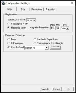
In the “Registration” box, define the orientation of the photo. If you used a registration image with a defined North point, select “North” for the “Initial Cursor Point.” Select if your North point in the photo is geographic or magnetic. If the latter, input the declination.

In the “Projection distortion” box, select a lens distortion or input custom values (see my previous post for instructions on computing these for your lens).

“Site” tab:

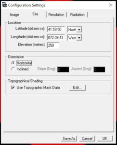
Input the coordinates of the image in the “Location” box. Note that we will use a common coordinate for all photos in the batch. This only works if there is not much distance between photos (I use 10km as a rule of thumb, but realistically, even 100km probably makes very little difference). If your sites are far apart, remember to set new coordinates for each cluster of neighboring sites.

If you ensure that your images point directly up as I suggest in my previous post, you should select “Horizontal” in the “Orientation” box. Note that in this case, “Horizontal” means “horizontal with respect to gravity” not “horizontal to the ground” which might not be the same thing if you are standing on a slope.

The “Topographic Shading” is not important if our only interest is estimating light. If you are interested in the canopy itself, this tool can be used to exclude a situation where, for instance, a tall mountain blocks light behind a canopy and would be considered a canopy element by the program.

“Resolution” tab:

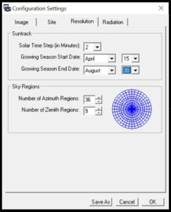
In the “Suntrack” box, it is important to carefully think about and set your season start and end dates. If you decide to consider other seasonal timespans later, you’ll need to rerun all of these analyses again. Remember that if you are estimating light during spring leaf-out or fall senescence, you’ll need to run separate analyses for each season with corresponding images.

“Radiation” tab:

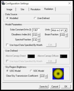
Assuming that you did not directly measure radiation values alongside your images, we need to model these parameters. These are probably the most difficult parameters to set because they will require some prior analysis from other data on radiation for your site.

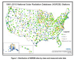
You can download radiation values from local observation points from the National Solar Radiation Dataset website. From these data, you can calculate parameter estimates for Cloudiness index, Beam fraction, and Spectral fraction. Remember only to use data for the seasonal window that matches the seasonal window of interest in your photos.

Cloudiness index (K_t):

This is essentially a measure of the percentage of the total radiation entering the atmosphere (H_o) that makes it to the ground surface (H) (i.e. not reflected by clouds).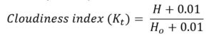

Where H is the Modeled Global Horizontal radiation (Glo Mod (W/m^2)) and H_o is the Hourly Extraterrestrial radiation (ETRN (W/m^2)) with 0.01 added to each to avoid dividing by zero.

Beam fraction (H_b/H):

Beam fraction is the ratio of radiation from direct beam (H_b) versus spectral radiation that reaches the ground (H). As you can imagine, as cloudiness increase, direct beam radiation decreases as it is diffused by the clouds; thus, we can estimate beam fraction as a function of cloudiness (K_t).

Where the constants -3.044 and 2.436 are empirically derived by Frazer et al. (1999) (see their paper for details and extensions).

Spectral fraction (R_p/R_s):

Spectral fraction is a ratio of photosynthetically active radiation wavelengths (R_p) to all broadband shortwave radiation (R_s). Frazer et al. (1999) provide the following equation for calculating Spectral fraction as a function of Cloudiness index (K_t).

Frazer et al. (1999) provide guidance on computing this as a monthly mean, but for most analyses, I think this overall average is probably fine.

The Solar constant is not region-specific, so the default value should be used.

The Transmission coefficient basically describes how much solar transmittance is expected on a perfectly clear day and is mainly a function of elevation and particulate matter in the air (i.e. dusty places have lower clear sky transmission). Frazer et al. (1999) suggest that this coefficient ranges from 0.4 to 0.8 globally and between 0.6 and 0.7 for North America. Therefore, they use a default of 0.65. Unless you have good reason to estimate your own transmission values, this default should be fine.

It can be very intimidating to pick values for these parameters. To be honest, I suspect that most practitioners never even open up the configuration menu, and instead, simply use the default parameters of the program. In the end, no matter what values you use to initialize your model, the most critical step is recording the values you chose and justifying your choice. As long as you are transparent with your analysis, others can repeat it and adjust these parameters in order to make direct comparisons with their own study system. Note: you can easily save this configuration file within GLA, too.

 5. Analyzing images

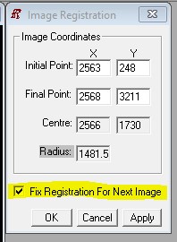
Once GLA is configured, you will need to register the first image. If you’ve named your registration image something like “AA000” as I have, it will be the first in your stack. Place the cursor on the known north point and drag to fit the circumference. Be sure to select the “Fix Registration for Next Image” button and also record the coordinate values for the circle.

Now that the first image is registered, we can automate the analysis process for the rest of the images. Unfortunately, GLA does not have a command line version and the GUI does not offer a method of batch processing. So, I wrote a script for the AutoHotKey program that replicates keyboard and mouse inputs. You can download AutoHotKey here. The free version is fine. For best operation, I recommend the 32-bit version.

I’ve included my AutoHotKey script below. You will need to use a text editor to edit the first line of the macro (line 17) with the file path to your image folder. Save the file as an AutoHotKey file (.ahk) and run it as administrator. Now you can pull up the GLA window and use the F6 shortcut to start the macro.

You should see the program move your cursor to open windows and perform operations, like in the video above. Since AutoHotKey is replicating mouse and keyboard movements, if you use your computer, it will stop the program. I suggest not touching your computer until the program is done (go get a cup of coffee while your new robot does all of your analysis for you!). If you must use your computer concurrently, you will need to first set up GLA and the AutoHotKey to run in a virtual machine.

#NoEnv
SetWorkingDir %A_ScriptDir%
CoordMode, Mouse, Window
SendMode Input
#SingleInstance Force
SetTitleMatchMode 2
#WinActivateForce
SetControlDelay 1
SetWinDelay 0
SetKeyDelay -1
SetMouseDelay -1
SetBatchLines -1

F6::
Macro1:
Loop, Files, ENTER_YOUR_FILEPATH_HERE*.*, F
{
WinMenuSelectItem, Gap Light Analyzer, , File, Open Image..
WinWaitActive, Gap Light Analyzer ahk_class #32770
Sleep, 333
ControlClick, Button1, Gap Light Analyzer ahk_class #32770,, Left, 1,  NA
Sleep, 10
WinWaitActive, Open file... ahk_class #32770
Sleep, 333
ControlSetText, Edit1, %A_LoopFileName%, Open file... ahk_class #32770
ControlClick, Button2, Open file... ahk_class #32770,, Left, 1,  NA
Sleep, 1000
Sleep, 1000
WinWaitActive, Gap Light Analyzer  ; Start of new try
Sleep, 333
WinMenuSelectItem, Gap Light Analyzer, , Configure, Register Image
WinWaitActive, Gap Light Analyzer  ahk_class ThunderRT5MDIForm
Sleep, 333
ControlClick, ThunderRT5CommandButton1, Gap Light Analyzer  ahk_class ThunderRT5MDIForm,, Left, 1,  NA
Sleep, 10
WinMenuSelectItem, Gap Light Analyzer, , View, OverLay Sky-Region Grid
WinMenuSelectItem, Gap Light Analyzer, , View, OverLay Mask
WinMenuSelectItem, Gap Light Analyzer, , Image, Threshold..
WinWaitActive, Threshold ahk_class ThunderRT5Form
Sleep, 333
ControlClick, ThunderRT5CommandButton1, Threshold ahk_class ThunderRT5Form,, Left, 1,  x34 y13 NA
Sleep, 10
WinMenuSelectItem, Gap Light Analyzer, , Calculate, Run Calculations..
WinWaitActive, Calculations ahk_class ThunderRT5Form
Sleep, 333
ControlClick, ThunderRT5CommandButton1, Calculations ahk_class ThunderRT5Form,, Left, 1,  NA
Sleep, 10
WinWaitActive, Calculation Summary Results ahk_class ThunderRT5Form
Sleep, 333
ControlSetText, ThunderRT5TextBox4, %A_LoopFileName%, Calculation Summary Results ahk_class ThunderRT5Form
ControlClick, ThunderRT5CommandButton2, Calculation Summary Results ahk_class ThunderRT5Form,, Left, 1,  NA
Sleep, 10
Sleep, 5000
}
MsgBox, 0, , Done!
Return

F8::ExitApp

F12::Pause

When the program has looped through all of the photos, a dialogue box will pop up with “Done!”

The data output is in a separate sub-window within GLA. It is usually minimized and hidden behind the registration image window. You can save the data, but GLA defaults to save the output as a semicolon delimited text file. This can be easily converted to a CSV or Excel worksheet in Excel.

And you’re done!

Be sure to check out my other posts about canopy research that cover the theory, hardware, field sampling, and analysis pipelines for hemispherical photos.

Also, check out my new method of canopy photography with smartphones and my tips for taking spherical panoramas.

---

References

Beckchafer, P. (2015). Hemispherical_2.0: Batch processing hemispherical and canopy photographs with ImageJ – User manual. doi:10.13140/RG.2.1.3059.4088.

Frazer, G. W., Canham, C. D., and Lertzman, K. P. (2000). Technology Tools: Gap Light Analyzer, version 2.0. The Bulletin of the Ecological Society of America 81, 191–197.

Frazer, G. W., Canham, C. D., and Lertzman, K. P. (1999). Gap Light Analyzer (GLA): Imaging software to extract canopy structure and gap light transmission indices from true-color fisheye photographs, users manual and documentation. Burnaby, British Columbia: Simon Fraser University Available at: http://rem-main.rem.sfu.ca/downloads/Forestry/GLAV2UsersManual.pdf.

Glatthorn, J., and Beckschäfer, P. (2014). Standardizing the protocol for hemispherical photographs: accuracy assessment of binarization algorithms. PLoS One 9, e111924.

Nobis, M. (2005). Program documentation for SideLook 1.1 – Imaging software for the analysis of vegetation structure with true-colour photographs. Available at: http://www.appleco.ch/sidelook.pdf.

Wilcox, S. (2012). National Solar Radiation Database 1991–2010 Update: User’s Manual. National Renewable Energy Laboratory Available at: https://www.nrel.gov/docs/fy12osti/54824.pdf.