I recently needed to learn text mining for a project at work. I generally learn more quickly with a real-world project. So, I turned to a topic I love: Wilderness, to see how I could apply the skills of text scrubbing and natural language processing. You can clone my Git repo for the project or follow along in the post below. The first portion of this post will cover web scraping, then text mining, and finally analysis and visualization.
Introduction
I thought it would be interesting to see how different Wilderness Areas are described. Having spent a lot of time in Wilderness Areas across the country, I know that they are extremely diverse. We can use text mining and subsequent analysis to examine just how that regional diversity is perceived and portrayed.
Wilderness.net provides a brief description, which I assume are written by the agency Wilderness managers, for each of the 803 designated Wilderness Areas in the United States [data disclaimer]. For example, here is the page for one of my favorite Wilderness Areas: South Baranof.
As always, we first load packages and set up the environment.
library(rvest) # For web scrapping
library(qdap) # For tagging parts of speech
library(tidytext) # Text mining
library(hunspell) # For word stemming
library(quanteda) # Text analsysis
library(cowplot) # Composite figures
library(ggrepel) # For text labels in visualizations
library(wordcloud2) # Word cloud vizualizations
library(tidyverse) # For everything.

# I find it easier to install wordcloud2 from the repo:
# library(devtools)
# devtools::install_github("lchiffon/wordcloud2")
Web scraping
I found the video tutorials here very helpful. In those tutorials, the author employs a Chrome extension, SelectorGadget to isolate the page elements that you want to scrape. Unfortunately, Wilderness.net uses an extremely convoluted page structure without CSS. Thus, I could not find a way to isolate the Wilderness descriptions using CCS tags. Instead, I scrub all of the body text and then use strsplit to cleave out the portions of the text I am interested in keeping.
Conveniently, each Wilderness Areas gets its own page on Wilderness.net and each of those pages are numbered consecutively in the page address. For example, South Baranof Wilderness is number 561: “wilderness.net/visit-wilderness/?ID=561”. This means that we can simply loop through each page, scrape the text, and store it for further analysis.
First, we need to set up an empty matrix that we will populate with the data we scrub from Wilderness.net. From the text, we want to isolate and store the Wilderness name, the state that contains the most acreage, the year of designation, the federal agency (or agencies) charged with its management, and the description text.
Colnames <- c("Wild", "State", "Year", "Agency", "Descrip")
WildText <- matrix(nrow = 804, ncol = length(Colnames))
colnames(WildText) <- Colnames
Now we loop through all of the pages to populate the empty matrix with our data.
for(i in 1:nrow(WildText)){
  link = paste0("https://wilderness.net/visit-wilderness/?ID=", i)
  page = read_html(link)
  content <- page %>%
    html_nodes("#maincontent , h1") %>%
    html_text()

  WildText[i, 1] <- content %>%
    strsplit("wilderness = '") %>%
    unlist() %>%
    `[`(2) %>%
    strsplit("';\nvar") %>%
    unlist() %>%
    `[`(1)

  WildText[i, 2] <- content %>%
    strsplit("stateAbbr = '") %>%
    unlist() %>%
    `[`(2) %>%
    strsplit("';\nvar") %>%
    unlist() %>%
    `[`(1)

  WildText[i, 3] <- content %>%
    strsplit("yearDesignated = '") %>%
    unlist() %>%
    `[`(2) %>%
    strsplit("';\nvar") %>%
    unlist() %>%
    `[`(1)

  WildText[i, 4] <- content %>%
    strsplit("agency = '") %>%
    unlist() %>%
    `[`(2) %>%
    strsplit(";\nvar") %>%
    unlist() %>%
    `[`(1) %>%
    gsub("[^a-zA-Z ]", "", .)

   WildText[i, 5] <- content %>%
    strsplit("<h2>Introduction</h2></div>") %>%
    unlist() %>%
    `[`(2) %>%
    strsplit("Leave No Trace\n\t\t\t") %>%
    unlist() %>%
    `[`(1) %>%
    strsplit(";\n\n\n") %>%
    unlist() %>%
    `[`(2)
}
Now we convert the matrix to a tibble and check to make sure our scraping rules captured all of the descriptions.
WildText <- as_tibble(WildText) # Convert the matrix to a tibble.

MissingDescrip <- WildText %>%
  mutate(WID = row_number()) %>%
  filter(is.na(Descrip)) %>%
  .$WID
In MissingDescrip we find that 44 Wilderness Areas are missing descriptions. So, we need to alter the rules a bit and re-scrape those pages.
for(i in MissingDescrip){
  link = paste0("https://wilderness.net/visit-wilderness/?ID=", i)
  page = read_html(link)

  WildText[i, 5] <- page %>%
    html_nodes("#maincontent") %>%
    html_text() %>%
    strsplit(paste0(";\nvar WID = '", i, "';\n\n\n")) %>%
    unlist() %>%
    `[`(2) %>%
    strsplit("Leave No Trace\n\t\t\t") %>%
    unlist() %>%
    `[`(1)
}
There are still a couple of Wildernesses with missing information: Wisconsin Islands Wilderness #654 and Okefenokee Wilderness #426. Each of these areas have idiosyncratic text elements, so we can write specific rules to pull the descriptions for each.
# Wisconsin Islands Wilderness #654
link = paste0("https://wilderness.net/visit-wilderness/?ID=", 654)
page = read_html(link)

WildText[654, 5] <- page %>%
  html_nodes("#maincontent") %>%
  html_text() %>%
  strsplit(";\nvar WID = '654';\n\n\n") %>%
  unlist() %>%
  `[`(2) %>%
  strsplit("Closed Wilderness Area") %>%
  unlist() %>%
  `[`(1)

# Okefenokee Wilderness #426
link = paste0("https://wilderness.net/visit-wilderness/?ID=", 426)
page = read_html(link)

WildText[426, 5] <- page %>%
  html_nodes("#maincontent") %>%
  html_text() %>%
  strsplit("WID = '426';\n\n\n") %>%
  unlist() %>%
  `[`(2) %>%
  strsplit("Leave No TracePlan Ahead and Prepare:") %>%
  unlist() %>%
  `[`(1)
The management of many Wilderness Areas is mandated to two agencies. We need to parse those.
WildText <- WildText %>%
  mutate(
    Agency = case_when(
      Agency == "Bureau of Land ManagementForest Service" ~ "Bureau of Land Management; Forest Service",
      Agency == "Bureau of Land ManagementNational Park Service" ~ "Bureau of Land Management; National Park Service",
      Agency == "Forest ServiceNational Park Service" ~ "Forest Service; National Park Service",
      Agency == "Fish and Wildlife ServiceForest Service" ~ "Fish and Wildlife Service; Forest Service",
      TRUE ~ Agency
    ),
    WID = row_number()
  ) %>%
  filter(!is.na(Wild))
It would be difficult to analyze 804-way comparisons. Instead, I want to group the Wilderness Areas by broad regions. I’m defining the Eastern Region as the states that boarder the Mississippi and those states to the east. The Western Region is everything to the west. Alaska, which contains almost half of the nation’s Wilderness acreage [link to post] is it’s own Region. I’ve grouped Hawaii and Puerto Rico into an Island Region, but because there are only 3 Areas in those places, we won’t have enough data to analyze.
WildText <- WildText %>%
  mutate(Region = case_when(State %in% c("MT", "CA", "NM", "WA", "NV", "AZ", "UT", "OR", "SD", "TX", "CO", "WY", "ND", "ID", "NE", "OK") ~ "West",
                            State %in% c("MN", "FL", "PA", "IL", "TN", "VA", "KY", "MO", "VT", "GA", "MI", "AR", "NJ", "MS", "WI", "LA", "NC", "SC", "ME", "IN", "AL", "WV", "NY", "NH", "MA", "OH") ~ "East",
                            State == "AK" ~ "Alaska",
                            State == "HI" | State == "PR" ~ "Island"))
At this point, I like to save these data so I don’t need to re-scrape every time I run the analysis. Next time, I can simply pick back up by redefining the WildText object.
saveRDS(WildText, "./WildernessDescriptions.rds")
WildText <- readRDS("./WildernessDescriptions.rds")
Text Mining
Now that we’ve successfully scrubbed our data, we can begin text mining. I found Silge & Robinson’s book, “Text Mining with R” invaluable.
There are a number of approaches to dealing with text that fall on a spectrum from relatively simple text mining to more complex natural language processing. For this exercise we will conduct a simple analysis that compares the words and their relative frequencies. To do so, we need to decompose the descriptions from word strings to individual words.
First, we remove non-text characters.
WT <- WildText %>%
  mutate(Descrip = gsub("\\.", " ", Descrip),
         Descrip = gsub("  ", " ", Descrip),
         Descrip = gsub("[^\x01-\x7F]", "", Descrip))
Next, we tag the parts of speech for each word in the essay.
WT$pos <- with(WT, qdap::pos_by(Descrip))$POStagged$POStagged

POS_list <- strsplit(WT$pos, " ") # Break string down into list of tagged words
Next, we create a tidy dataframe of the parts of speech and retain only the informational words (nouns, verbs, adjectives, and adverbs). We also remove “stop words” or common words that tend not to provide a strong signal (or the wrong signal).
WT2 <- data.frame(Wild = rep(WT$Wild, sapply(POS_list, length)), words = unlist(POS_list)) %>% # Convert lists of tagged words into tidy format, one word per row
  separate(words, into = c("word", "POS"), sep = "/") %>% # Create matching columns for the word and the tag
  filter(POS %in% c("JJ", "JJR", "JJS", "NN", "NNS", "RB", "RBR", "RBS", "VB", "VBD", "VBG", "VBN", "VBP", "VBZ")) %>% # Keep only the nouns, verbs, adjectives, and adverbs
  anti_join(stop_words) # Remove stop words
Next we lemmatize the words (i.e. extract the stem word, for instance, peaks = peak and starkly = stark).
WT2$stem <- NA
for(i in 1:nrow(WT2)){
  WT2$stem[i] <- hunspell_stem(WT2$word[i]) %>% unlist() %>% .[1]
  print(paste0(sprintf("%.2f", i/nrow(WT2)), "% completed")) # This just outputs a progress indicator.
}
Finally, we can add the regions from the original dataset onto the tidy dataset and save the data object for future use.
WT2 <- WT2 %>%
  left_join(WildText %>% select(Wild, Region))
At this point, I like to save these data so we don’t need to reprocess every time we run the analysis.
# saveRDS(WT2, "./WildernessByWord.rds")
WT2 <- readRDS("./WildernessByWord.rds")
Analysis and Visualization
After all that effort of scraping text from the web and text mining, we can finally begin to take a look at our data. One of the first questions one might as is: do managers tend to write longer descriptions for Areas depending on the region?
WT2 %>%
  group_by(Region, Wild) %>%
  summarise(WordCount = length(word)) %>%
  ggplot(aes(x = fct_reorder(Region, WordCount, median), col = Region, y = WordCount)) +
  geom_jitter(size = 3, alpha = 0.4, pch = 16, height = 0) +
  geom_boxplot(width = 0.3, alpha = 0.7) +
  scale_y_log10() +
  scale_color_manual(values = c("#008dc0", "#8ba506", "grey", "#bb5a00"))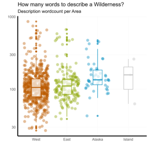
Descriptions of Alaskan Wilderness Areas tend to be longer than those for other regions. While descriptions for Areas in Hawaii and Puerto Rico also have a high median, there are too few to make strong comparisons.
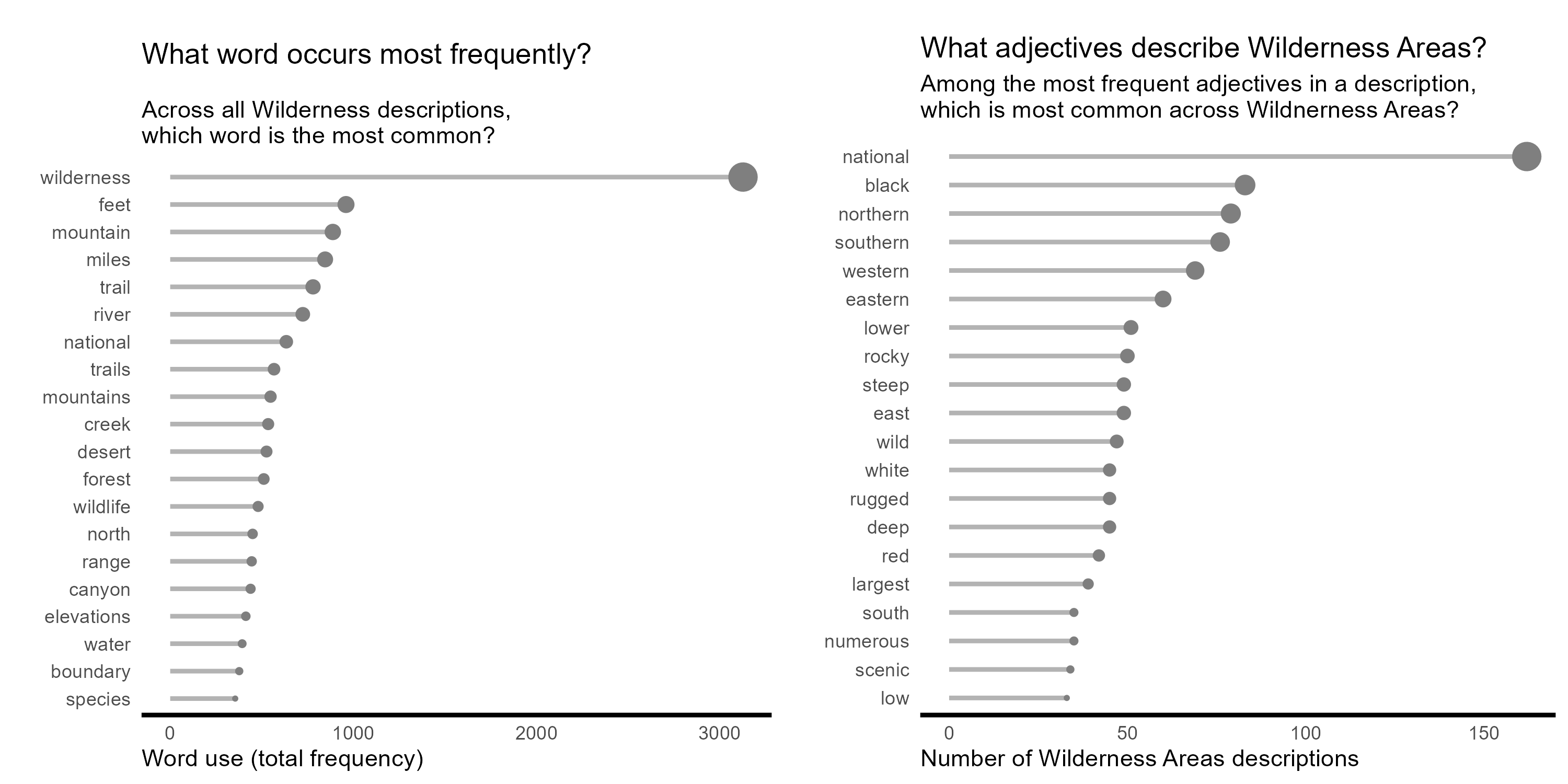
Another common question is: which words are used most frequently? We can answer that most simply by looking for the word with the high use count across all descriptions.
 WT2 %>%
    group_by(word) %>%
    tally() %>%
    arrange(desc(n)) %>%
    top_n(20)
Unsurprisingly, “wilderness” is the most frequently used word, by far. Factual descriptors like “feet”, “miles”, “elevation”, and “boundary” are common. Features like “mountain”, “trail”, “river”, “wildlife”, “dessert”, and “forest” are also common.
Interestingly, no emotive adjectives make the list. John Muir would be disappointed! We can also pull out only the adjectives.
WT2 %>%
    filter(POS %in% c("JJ", "JJS", "JJR")) %>%
    group_by(word, Wild) %>%
    tally() %>%
    group_by(Wild) %>%
    filter(n == max(n)) %>%
    group_by(word) %>%
    tally() %>%
    arrange(desc(n)) %>%
    top_n(20)
Other than the prosaic “national” and direction words, we can see some descriptor of the sublime, like “steep”, “rugged”, “rocky”, and “wild” that would make the transcendentalists progenitors of the wilderness concept proud.
To make the main figure for this project, I really wanted to use word clouds. Word clouds aren’t a great visualization for data interpretation, but they are a fun gimmick and make for interesting visuals!
Unfortunately, R doesn’t have the best support for generating fancy wordclouds. The package wordcloud is solidly reliable, but can only make very basic images. The package wordcloud2 allows for far more customization, but it is extremely buggy and requires some work-arounds on most systems.
I want the regional word clouds to conform to the Region’s shape. I made some simple shape images (here: East, West, Alaska) that we can pass to wordcloud2.
Depending on your system, the image may not populate in RStudio’s plotting window. If you don’t see the plot, try clicking the button to “show in new window” which will open a browser tab. Try refreshing the browser tab a few times until the wordcloud generates. Unfortunately, there is no way to constrain the aspect ratio of the cloud, so you will need to resize your browser window to a square. Then you can right-click and save the image. …like I said, wordcloud2 requires far too many work-arounds, but it is the only option for word clouds with custom shapes in R.
Below I’m showing the code for generating the Western region. It should be easy to alter for the other regions (all of the code is on github).
WT2 %>%
  filter(Region == "West") %>%
  filter(word != "wilderness") %>%
  count(word) %>%
  filter(n > 10) %>%
  wordcloud2(figPath = "./West.png",
             maxRotation = 0,
             minRotation = 0,
             color = "#bb5a00",
             fontFamily = 'serif')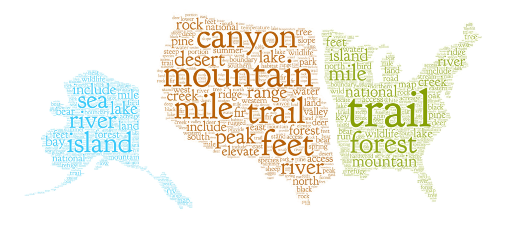
I pulled the wordclound images into Illustrator to make the final adjustments. (You could certainly do all of this in R, but I’m much faster at Illustrator and prefer to use a visual program for graphic design decisions.)
Because wordclouds are not useful for quantitative interpretation, I also want to make some histograms of the most common words associated with each region. Again, I’m only showing code for the Western region below, all of the code is on Github.
WT2 %>%
  filter(Region == "West") %>%
  filter(stem != "wilderness") %>%
  count(stem) %>%
  arrange(desc(n)) %>%
  top_n(40) %>%
  ggplot(aes(x = fct_reorder(stem, n), y = n)) +
  geom_bar(stat = "identity", fill = "#bb5a00", width = 0.7) +
  coord_flip() +
  labs(y = "", x = "") +
  theme(axis.text.y = element_text(color = "#bb5a00"),
        axis.line.y = element_blank(),
        panel.grid.major = element_blank(),
        axis.text = element_text(family = "serif"))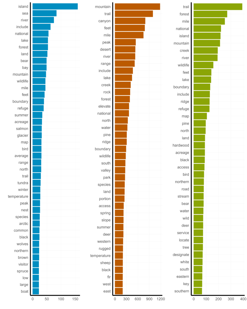
Another question we could ask is: which words most distinguish regions from other regions? For example, “mountain” and “trail” are high frequency words in the Western region, but they also occur at high frequency in the Eastern region, as well. So, these terms don’t help us distinguish between regions. Instead we can estimate log ratios of word occurrence between regions. Log ratios conveniently scale symmetrically around zero. Greater absolute values indicate words particularly relevant to one region and smaller values indicate words that are equally relevant to both regions.
wordratios <- WT2 %>%
  filter(word != "wilderness") %>%
  filter(Region == "East" | Region == "West") %>%
  count(stem, Region) %>%
  filter(sum(n) > 10) %>%
  ungroup() %>%
  spread(Region, n, fill = 0) %>%
  mutate_if(is.numeric, funs((. + 1)/sum(. + 1))) %>%
  mutate(logratio = log(East/West)) %>%
  arrange(desc(logratio))

wordratios %>%
  arrange(abs(logratio)) # Small log ratios indicate terms that are equally likely to be from East or West

WT2 %>%
  count(stem, Region) %>%
  group_by(stem) %>%
  filter(sum(n) >= 10) %>%
  ungroup() %>%
  pivot_wider(names_from = Region, values_from = n, values_fill = 0) %>%
  mutate_if(is.numeric, list(~(. + 1) / (sum(.) + 1))) %>%
  mutate(logratio.EW = log(East / West)) %>%
  arrange(abs(logratio.EW)) %>%
  slice(1:20) %>%
  mutate(class = "mid") %>%
  bind_rows(
    WT2 %>%
      count(stem, Region) %>%
      group_by(stem) %>%
      filter(sum(n) >= 10) %>%
      ungroup() %>%
      pivot_wider(names_from = Region, values_from = n, values_fill = 0) %>%
      mutate_if(is.numeric, list(~(. + 1) / (sum(.) + 1))) %>%
      mutate(logratio.EW = log(East / West)) %>%
      arrange((logratio.EW)) %>%
      slice(1:20) %>%
      mutate(class = "west")
  ) %>%
  bind_rows(
    WT2 %>%
      count(stem, Region) %>%
      group_by(stem) %>%
      filter(stem != "roger") %>%
      filter(sum(n) >= 10) %>%
      ungroup() %>%
      pivot_wider(names_from = Region, values_from = n, values_fill = 0) %>%
      mutate_if(is.numeric, list(~(. + 1) / (sum(.) + 1))) %>%
      mutate(logratio.EW = log(East / West)) %>%
      arrange(desc(logratio.EW)) %>%
      slice(1:20) %>%
      mutate(class = "east")
  ) %>%
  ggplot(aes(x = fct_reorder(stem, logratio.EW),
             y = logratio.EW,
             col = class)) +
  geom_segment(aes(xend = fct_reorder(stem, logratio.EW),
                   y = case_when(class == "west" ~ -0.1,
                                 class == "mid" ~ 0,
                                 class == "east" ~ 0.1),
                   yend = logratio.EW)) +
  geom_point(data = . %>% filter(class == "west"), aes(size = exp(abs(logratio.EW))), pch = 16) +
  geom_point(data = . %>% filter(class == "east"), aes(size = exp(abs(logratio.EW))), pch = 16) +
  geom_text(data = . %>% filter(class == "west"), aes(label = stem, y = 0), hjust = 0) +
  geom_text(data = . %>% filter(class == "east"), aes(label = stem, y = 0), hjust = 1) +
  geom_text(data = . %>% filter(class == "mid"), aes(label = stem, y = 0)) +
  coord_flip() +
  scale_color_manual(values = c("#8ba506", "grey70", "#bb5a00")) +
  theme(axis.text.y = element_blank(),
        axis.line.y = element_blank(),
        panel.grid.major = element_blank()) +
  labs(x = "",
       y = "Log ratio ('Uniqueness' of words for a region)",
       title = "Which words are most unique to a Wilderness?")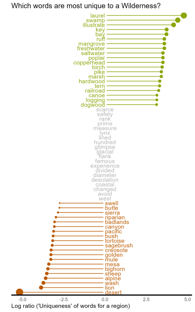
In the image above we can see the 20 most unique words that distinguish the Eastern from the Western regions. “Laurel”, “swamp”, “key”, and “bay” are characteristic of the East while “desert”, “lion”, “wash”, and “alpine” are almost exclusively used to describe Western areas. Words like “safety”, “coastal”, and “glimpse” are commonly used in both regions. Interestingly, the word “west” is used commonly in Eastern descriptions. I was also surprised to see “lynx” and “glacial” to be equally common.
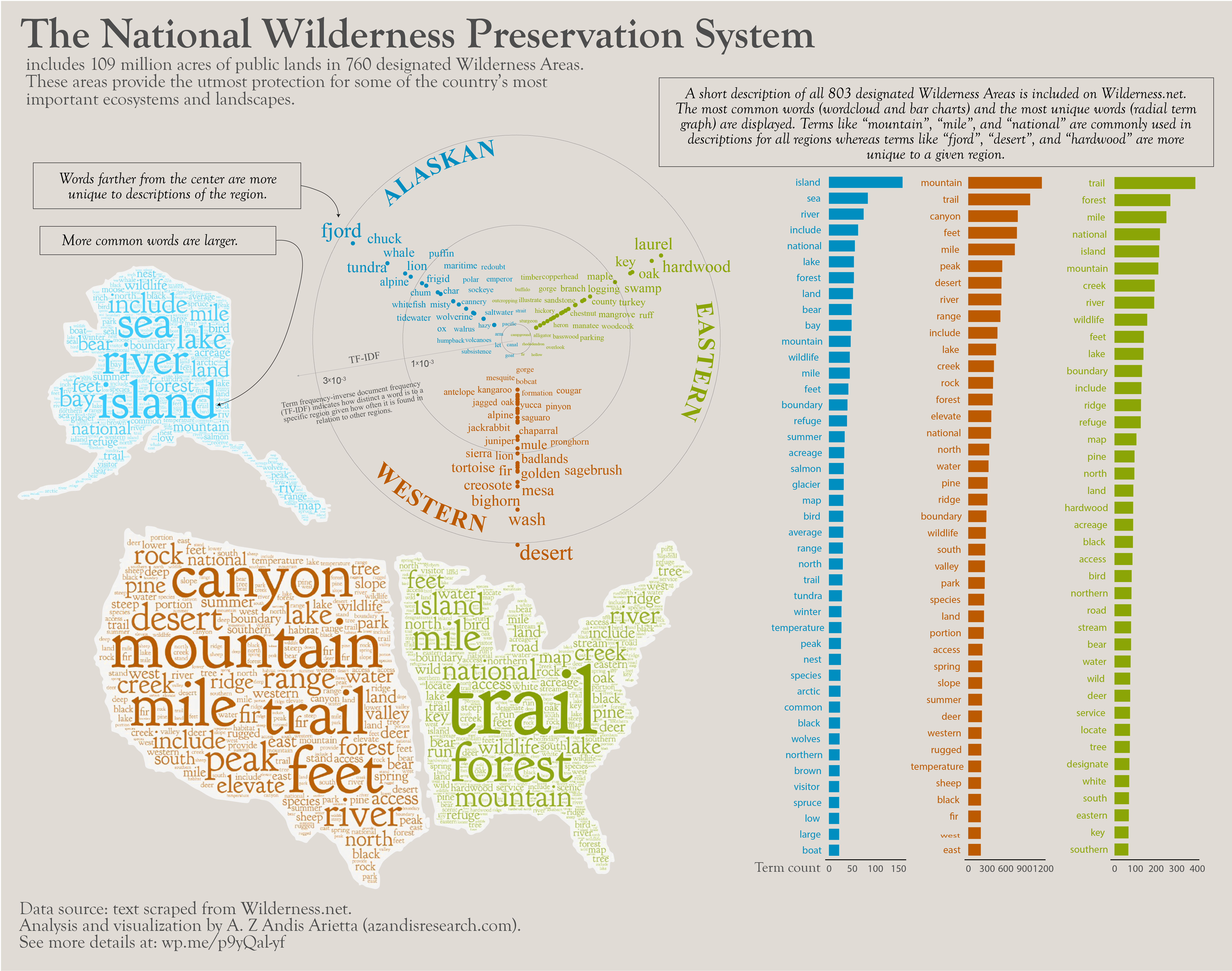
Log ratios aren’t as useful when we have more than two groups to compare. In our case, where we want to compare multiple groups (i.e. West, East, and Alaska), we can find the words that most distinguish one region from the others by computing the term frequency-inverse document frequency (tf-idf). This metric is computed by multiplying the the number of times a word is used in a given “document” by the inverse of that word’s frequency across all “documents”. In this case, we treat all descriptions from a region as a single “document”. Similar to log ratios, tf-idf let’s us know how relevant a term is to a given document, but allows us to compare across many documents.
WT2 %>%
  filter(Region != "Island") %>%
  filter(!is.na(stem)) %>%
  filter(stem != "roger") %>%
  count(Region, stem, sort = TRUE) %>%
  bind_tf_idf(stem, Region, n) %>%
  group_by(Region) %>%
  top_n(10, tf_idf) %>%
  arrange(desc(Region), desc(tf_idf)) %>%
  print(n = 40)
# A tibble: 32 x 6
# Groups: Region [3]
Region stem n tf idf tf_idf
1 West desert 533 0.00852 0.405 0.00346
2 West wash 125 0.00200 1.10 0.00220
3 West bighorn 95 0.00152 1.10 0.00167
4 West mesa 90 0.00144 1.10 0.00158
5 West golden 79 0.00126 1.10 0.00139
6 West creosote 78 0.00125 1.10 0.00137
7 West fir 203 0.00325 0.405 0.00132
8 West sagebrush 73 0.00117 1.10 0.00128
9 West tortoise 71 0.00114 1.10 0.00125
10 West badlands 63 0.00101 1.10 0.00111
11 East laurel 38 0.00180 1.10 0.00198
12 East hardwood 90 0.00427 0.405 0.00173
13 East key 68 0.00323 0.405 0.00131
14 East oak 66 0.00313 0.405 0.00127
15 East illustrate 20 0.000949 1.10 0.00104
16 East swamp 53 0.00251 0.405 0.00102
17 East logging 37 0.00175 0.405 0.000712
18 East maple 34 0.00161 0.405 0.000654
19 East turkey 34 0.00161 0.405 0.000654
20 East branch 33 0.00157 0.405 0.000635
21 Alaska fjord 17 0.00243 1.10 0.00267
22 Alaska anchorage 11 0.00157 1.10 0.00173
23 Alaska tundra 28 0.00400 0.405 0.00162
24 Alaska prince 9 0.00128 1.10 0.00141
25 Alaska wale 9 0.00128 1.10 0.00141
26 Alaska chuck 8 0.00114 1.10 0.00125
27 Alaska whale 20 0.00286 0.405 0.00116
28 Alaska lion 17 0.00243 0.405 0.000984
29 Alaska alpine 16 0.00228 0.405 0.000926
30 Alaska cook 5 0.000714 1.10 0.000784
31 Alaska frigid 5 0.000714 1.10 0.000784
32 Alaska warren 5 0.000714 1.10 0.000784Words like “desert”, “wash”, “bighorn”, and “mesa” are highly indicative of the West. The East is described most distinctly by it’s plant species: “laurel”, “oak”, “maple” and by terms like “key” which refers to the islands in the southeast. Alaska is dominated by intuitive terms like “fjord”, “tundra” and “alpine” and sea animals like “whale” and sea “lion”. Place names also rise to high relevance for Alaska with terms like “Anchorage”, “Prince of Wales Island”, and “Cook Inlet”.
When plotting differences between East and West in log-ratios, above, it made sense to use a diverging bar graph (or lollipop graph, specifically). But with more than a two-way comparison, visualization gets more complicated.
After a few iterations, I settled on visualizing the most distinctive terms (i.e. terms with highest tf-idf) as growing larger from a common point. I accomplished this by wrapping the plot around a circular coordinate system. Terms that are larger and further from the axes of other regions are more distinctive to the focal region.
Before plotting, I also remove the words associated with proper noun place names.
WT2 %>%
  filter(Region != "Island") %>%
  filter(!is.na(stem)) %>%
  filter(!stem %in% c("roger", "anchorage", "prince", "wale", "cook", "warren", "admiralty", "coronation")) %>%
  count(Region, stem, sort = TRUE) %>%
  bind_tf_idf(stem, Region, n) %>%
  group_by(Region) %>%
  top_n(30, tf_idf) %>%
  ungroup() %>%
  mutate(ordering = as.numeric(as.factor(Region)) + (tf_idf*100),
         stem = fct_reorder(stem, ordering, .desc = FALSE)) %>%
  mutate(tf_idf = tf_idf * 100) %>%
  ggplot(aes(x = fct_relevel(Region, c("East", "West", "Alaska")), label = stem, y = tf_idf, col = Region)) +
  geom_point() +
  coord_flip() +
  scale_color_manual(values = c("#008dc0", "#8ba506", "#bb5a00")) +
  scale_y_log10(limits = c(.025, 0.35)) +
  coord_polar() +
  geom_text_repel(aes(cex = tf_idf), max.overlaps = 100, family = "serif", segment.linetype = 0) +
  theme(panel.grid.major.x = element_blank(),
        axis.line = element_blank(),
        axis.text = element_blank()) +
  labs(x = "", y = "")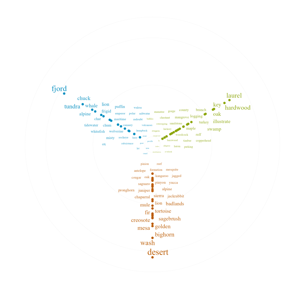
With all of the components created, I pulled everything into Illustrator to design the final infographic.
There is certainly a lot more that one could learn from these data. For instance, do descriptions differ by management agency? Would we find stronger divergence in language used to describe North versus South regions in the lower 48 rather than East-West? Nevertheless, this was a useful exercise for learning a bit more about web scrapping, text mining, and word analysis.