Every once in a while, I come across a plot form that is not in my ggplot repertoire. For example, I occasionally want to make a funnel plot in my work. I’m ashamed to admit that I usually pop over to Illustrator to make those plots.

But last week, a friend asked me if I knew how to make biomass pyramids in ggplot2. Since I love a challenge and a pyramid plot is just an upside down funnel, I figured I would give it a try.

My solution was to hack the geom_bar() functionality to make a mirrored bar plot, then flip the axis.

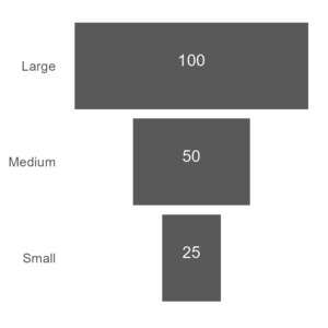
Here’s a simple example with some simulated data:

library(tidyverse)

X <- data.frame(level = c("Small", "Medium", "Large"), value = c(25, 50, 100)) 

X %>%
  ggplot(aes(x = fct_reorder(level, value), y = value)) +
  geom_bar(
    stat = "identity", 
    width = 0.9
    ) +
  geom_bar(
    data = . %>% mutate(value = -value),
    stat = "identity",
    width = 0.9
    ) +
  geom_text(aes(label = value, y = 0),
            col = "white",
            vjust = 0) +
  coord_flip() +
  theme_minimal() +
  theme(
    axis.title = element_blank(),
    panel.grid = element_blank(),
    axis.text.x = element_blank()
    )

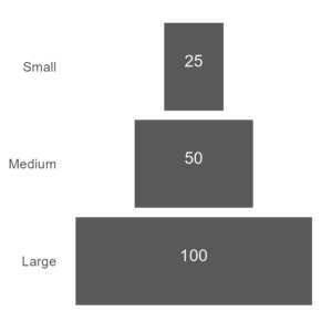
If you want a pyramid instead of a funnel, just change value to -value when passing the x = fct_reorder(level, -value) argument to aes().

There is a lot you can do to customize the plots from this basic plot. As an example, I decided to loosely replicate the biomass pyramid example image from Wikipedia.

library(cowplot)

Biomass <- data.frame(System = c(rep("Aquatic Ecosystem", 4), rep("Terrestrial Ecosystem", 4)),
                      level = c("Sea Lion", "Herring", "Zooplankton", "Phytoplankton", "Snakes", "Mice", "Grasshoppers", "Grasses"),
                      value = c(1e3, 1e4, 1e5, 1e6, 15.2, 152, 1520, 15200))

Aqua <- Biomass %>%
  filter(System == "Aquatic Ecosystem") %>%
  mutate(value = log10(value)) %>%
  ggplot(aes(x = fct_reorder(level, -value), y = value, fill = as.numeric(fct_reorder(level, abs(value))))) +
  geom_bar(
    stat = "identity", 
    width = 1) +
  geom_bar(
    data = . %>% mutate(value = -value),
    stat = "identity",
    width = 1
  ) +
  geom_text(aes(label = paste0(10^value, " kg"), y = 0),
            col = "goldenrod",
            vjust = 3,
            cex = 4) +
  geom_text(aes(label = level, y = 0),
            col = "grey",
            vjust = 0,
            cex = 8) +
  coord_flip() +
  theme_minimal() +
  theme(
    axis.title = element_blank(),
    panel.grid = element_blank(),
    axis.text = element_blank(),
    legend.position = "none"
  ) +
  scale_fill_gradient(low = "dodgerblue", high = "navyblue") +
  labs(title = "Aquatic Ecosystem")

Terra <- Biomass %>%
  filter(System == "Terrestrial Ecosystem") %>%
  mutate(value = log10(value)) %>%
  ggplot(aes(x = fct_reorder(level, -value), y = value, fill = as.numeric(fct_reorder(level, abs(value))))) +
  geom_bar(
    stat = "identity", 
    width = 1) +
  geom_bar(
    data = . %>% mutate(value = -value),
    stat = "identity",
    width = 1
  ) +
  geom_text(aes(label = paste0(10^value, " kg"), y = 0),
            col = "goldenrod",
            vjust = 3,
            cex = 4) +
  geom_text(aes(label = level, y = 0),
            col = "grey",
            vjust = 0,
            cex = 8) +
  coord_flip() +
  theme_minimal() +
  theme(
    axis.title = element_blank(),
    panel.grid = element_blank(),
    axis.text = element_blank(),
    legend.position = "none"
  ) +
  scale_fill_gradient(low = "palegreen", high = "darkgreen") +
  labs(title = "Terrestrial Ecosystem")

plot_grid(
  Aqua,
  Terra,
  nrow = 1
)

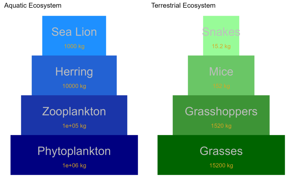
A few notes on this plot, to remove the space between bars use width = 1 in geom_bar().

You’ll also see that I decided to log-scale the values. You have to transform the data before piping it into the ggplot function, otherwise when we make the values negative, the log is undefined.

I also decided to color the bars. In order to get the gradient to scale correctly, we need to order the levels factor when we pass it to the fill argument.

I tried valiantly to make side-by-side figures using facet_wrap() and scales = "free", but found it difficult to get the factor level order correct for the color fill. So, I fell back to making separate plots and paneling them together with cowplot.