Despite the fact that foresters have been estimating forest canopy characteristics for over a century or more, the techniques and interpretation for these measurements is surprisingly inconsistent. As part of my dissertation research, I wanted to ask what I thought was a simple question: “How much light reaches different vernal pools over the season?” It took a lot of literature searching, a lot of emails, and a lot of trial and error to discover that this is actually not as simple of a question as I originally thought.

But in the end, I’ve developed what I think is a very sound workflow. In the hopes of saving other researchers a journey through the Wild West of canopy-based light estimates, I decided to publish my notes in a series of blog posts.

• In this first post, I’ll cover the rationale behind hemispherical photo measurements.
• The second post will compare hardware and address measuring/calibrating lens projections.
• The third post will focus on capturing images in the field.
• Finally, the fourth post will be a detailed walk-through of my software and analysis pipeline, including automation for batch processing multiple images.

Why measure light with hemispherical photos?

Light is an important environmental variable. Obviously the light profile in the forest drives photosynthesis in understory plants, but it is also important for exothermic wildlife, and can also impact abiotic factors like snow retention. An ecologist interested in any of these processes should be interested in the light environment at specific points in the habitat. Although light intensity at a point can be measured directly with photocells (Getz 1968), this requires continuous measurement at each point of interest over the entire seasonal window of interest. For most applications, this would be intractable. A more common method involves measuring the canopy above a point and estimating the amount of sky that is obstructed in order to infer the amount of light incident at that location.

Fortunately, since both foresters and ecologists are interested in the canopy, the field has produced a multitude of resources for measuring it. However, foresters are more often interested in estimating the character of the canopy itself and the canopy metrics they use are not always directly relatable to questions in ecology.

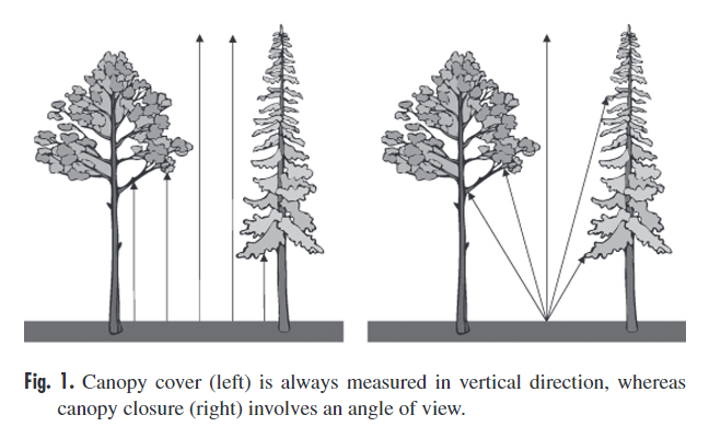
For instance, while foresters are generally interested in canopy COVER, ecologists might be more interested in canopy CLOSURE. These terms are similar enough that they are often (incorrectly) used interchangeably. According to Korhonen (2007) and Jennings et al. (1999), canopy cover is “the proportion of the forest floor covered by the vertical projection of the tree crowns” while canopy closure is “the proportion of sky hemisphere obscured by vegetation when viewed from a single point” (see the figure below).

The choice between measuring cover versus closure depends on both the scale and perspective of your research. For instance, forest-wide measurements of photosynthetic surface will probably be estimated from remote sensing data which is a vertical projection (i.e. canopy cover). However, if you are interested in the amount of light reaching a specific understory plant or a vernal pool, canopy closure is more relevant.

The disparity in perspective can be an issue in downstream analysis too. For instance, some analysis procedures consider only the outer edge of a tree crown or contiguous canopy and ignore gaps within this envelope. This kind of analysis is much less useful if your interest is in the light filtering through canopy gaps.

Canopy estimation:

There are three main ways to estimate canopy characteristics: direct field measurements, indirect modelling from other parameters, and remote sensing. The choice of measurement methods employed will largely be determined by the scope of the question and the scale-accuracy required. For the purpose of my research, I am interested in estimating light environments for a specific set of vernal pools; so, direct measurements are most useful. However, if I wanted to know how different tree composition influences light environments of ponds on average across forest habitats, I might want to try modelling that relationship followed by ground-truthing with direct measurements.

The rest of this post will focus on directly measuring canopy closure to estimate light environments.

Measurement methods:

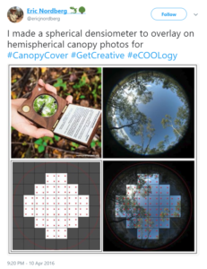
The most popular methods for directly measuring closure are hemispherical photography and spherical densiometer. A spherical densiometer (Lemmon 1956) is basically a concave or convex mirror that reflects the entire canopy. A grid is drawn over the mirror and researchers can count the number of quadrants of sky versus canopy.

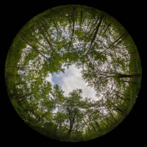
Hemispherical photos use a similar principle. A true hemispherical lens projects a 180 degree picture of the canopy that can then be processed to determine percentage of sky versus canopy.

Advantages of densiometer are that they are cheap, easy to operate, and can function in any light conditions. The exact converse is true of hemispherical photography which can be expensive, difficult to operate, and requires very narrow light conditions (I’ll get into the particulars in post 3).

So, why would anyone use hemispherical photos over densiometers?

The main disadvantage of a densiometer is that the estimates are instantaneous, whereas hemispherical photos can be integrated to estimate continuous measurements. It is easiest to explain this with an example.

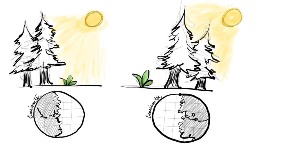
Imagine you want to know how much light is received by a specific plant on the forest floor at the very edge of a clearcut (see figure below). A closure estimate from a densiometer would indicate 50% closure no matter the orientation of the tree line. However, if that little plant is in the northern hemisphere, we know that it will receive much less light if the clearcut lies to the north than if the clearcut lies to the south due to the angle and orientation of the sun.

The advantage of hemispherical photos (if taken with known orientation and location) is that they can be used to integrate light values over time with respect to the direction of the sun relative to gaps in the canopy. This means that with a single photo (or two photos for deciduous canopies) one can calculate the path of the sun and estimate the total light received by the plant in our example at any point in time or cumulatively over a range of time.

An ancillary advantage of photos is that they can be archived along with the scripts used for processing, which makes the entire analysis easily reproducible.

I’ll go much further in depth in later posts, but as a preview, here is a general overview of how light estimates are calculated from hemispherical photos:

1. Hemispherical photos are captured in the field at a specific location and known compass orientation.
2. Images are converted to binary, such that each pixel is either black or white using thresholding algorithms.
3. Software can then be used to project a sun path onto the image.
4. Models parameterized with average direct radiation, indirect radiation, and cloudiness can then estimate the total radiation filtering through the gaps represented as white pixels in the photo at any point in time or averaged over time ranges.
5. The result is a remarkably accurate point estimate of incident light at any time in the season.

I’ll be drafting subsequent post in the coming weeks so be sure to check back in!

Be sure to check out my other posts about canopy research that cover the theory, hardware, field sampling, and analysis pipelines for hemispherical photos.

Also, check out my new method of canopy photography with smartphones and my tips for taking spherical panoramas.

---

References:

Getz, L. L. (1968). A Method for Measuring Light Intensity Under Dense Vegetation. Ecology 49, 1168–1169. doi:10.2307/1934505.

Jennings, S. B., Brown, N. D., and Sheil, D. (1999). Assessing forest canopies and understorey illumination: canopy closure, canopy cover and other measures. Forestry 72, 59–74. doi:10.1093/forestry/72.1.59.

Korhonen, L., Korhonen, K. T., Rautiainen, M., and Stenberg, P. (2006). Estimation of forest canopy cover: a comparison of field measurement techniques. Available at: http://www.metla.fi/silvafennica/full/sf40/sf404577.pdf.

Lemmon, P. E. (1956). A Spherical Densiometer For Estimating Forest Overstory Density. For. Sci. 2, 314–320. doi:10.1093/forestscience/2.4.314.